TRAFFIC CLASSIFIER
Overview
For this project for CS 4516: Advanced Computer Networks, I worked with a partner to implement an Internet Protocol (IP) gateway that intercepts traffic from an Android x86 6.0 virtual machine, separates packets into flows, and uses a random forest classifier to predict which application they came from, despite the packet payloads being encrypted.
This project was inspired by a paper we read for class. In the paper, researchers describe a framework, called AppScanner, for classifying encrypted smartphone network traffic, and correlating flows to specific applications.
This project shows that traffic classification is still possible despite the use of encryption. Even without knowing the specific contents of packets, you can still perform fingerprinting based on various features of the encrypted flows.
We were able to reimplement a small part of what the researchers made for AppScanner, and achieved acceptable accuracy for a small set of test applications.
Phase 1
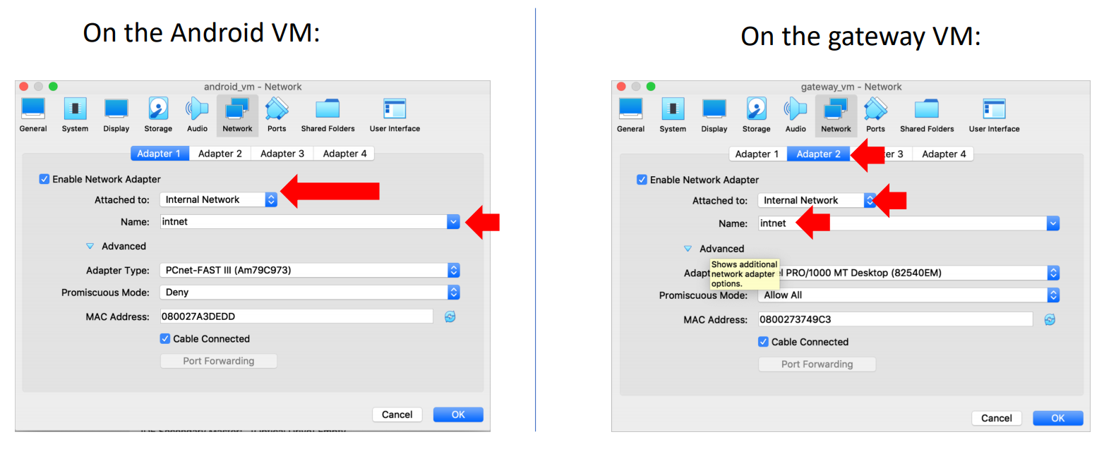
For this phase, we configured a TinyCore VM to act as a gateway. We set up an SSH connection to the virtual machine from the host machine and configured the Android x86 6.0 and TinyCore VMs to work on the same virtual network.
IP Gateway
Next, we configured the eth1 interface of TinyCore to have the static IP address 192.168.12.1, netmask 255.255.255.0. This is the interface that connects to the Internet. TinyCore's other (virtual) interface, eth0, will be hooked up to the Android VM. We also used iptables to route packets from eth0 to the Internet and dback. Now TinyCore can act like a gateway middlebox.
DHCP Server
We also wanted TinyCore to act as a DHCP server for its subnet. We used the program udhcpd with this configuration file to do that:
Startup Script
Finally, we needed to persist these changes so they apply every time the TinyCore VM reboots. We wrote this script, /opt/eth1.sh, to run at startup and apply all the configurations. This script kills the udhcpc process if it's already running, configures eth1 interface, and then starts the udhcpc server process.
Phase 2
For this phase, we wrote a Python script called logFlows that captures packets from the Android VM and separates them into bursts and flows. A flow is defined as a sequence of packets with the same source IP, source port, destination IP, and destination port. A burst is a group of flows separated by gaps of greater than one second of silence. After each burst, the program prints a report on which each flow in that burst, in the following format:
As our program is capturing packets, we record each "half" flow, which is the traffic going in a single direcction. At the end of a burst, we match each half flow to its corresponding half flow in order to create a "full" flow which encapsulates all of the traffic going between two hosts.
We have a daemon process that runs in the background in order to detect the end of a burst during live packet capture. This process checks every fifth of a second to see if the last packet received is over one second old. If this is the case, the recorded half flows are matched into full flows and the statistics for each flow are printed to the standard output.
logFlows uses Python 2 and requires the Python package scapy, which can be easily installed with pip. Note that it must be run as root on TinyCore.
Phase 3
In phase 3, we implemented an offline machine learning classifier. We wrote a script, pcapper.py, that runs on the TinyCore gateway VM, captures packets from eth1, and writes them to PCAP files. Another script, trainer.py, builds a classification model based on the feature vectors described below. The final script, ClassifyFlows, takes in a PCAP packet trace and the model created by trainer.py, and attempts to identify which application each flow in the PCAP file came from.
Classification Vectors
While we were in the process of trying to make the machine learning component as accurate as possible, we continually added features in the hopes of improving the accuracy of the model. Our feature vector originally contained only five elements, and expanded to fourteen elements as we iterated on our strategy for machine learning.
The following measurements were elements of the feature vector:
- Byte ratio (bytes sent / bytes received, or reciprocal)
- Packet ratio (packets sent / packets received, or reciprocal)
- Mean packet length
- Standard deviation of packet lengths (zero if n ≤ 2)
- Packet length kurtosis
- Packet length skew
- Mean time gap between each packet (zero if n ≤ 1)
- Time gap kurtosis
- Time gap skew
- Min packet length
- Max packet length
- Min time gap
- Max time gap
- Protocol (1 for TCP, 0 for UDP)
As you can see from the list above, the bulk of the features are statistical measures for two main lists. The first list is simply the lengths of all the packets in the flow. The second list is the gaps of time between each packet arrival. Because this list records the intervals, if there were only two packets in a flow this list would be only one item long.
Test Data
We collected four rounds of packets traces for each of the applications being tested. Each round of training data collection took around thirty minutes to an hour. Certain applications generated many megabytes of data. This was especially true for applications that regularly streamed video, such as YouTube. Other applications generated far less traffic, such as Fruit Ninja, which played ads at relatively infrequent intervals. In total, we collected 314 MiB of data in order to train our classifier.Classification Model
Our first attempt at a classification model used support vector classification. The implementation of this classifier in sklearn currently has issues with data containing very large and very small numbers; the classifier took many minutes to train instead of seconds. Because of this, it was difficult to work with as we rapidly collected more data to train our model. We tried to do our own normalization, but this did not help appreciably.
Because of these difficulties, we moved to a random forest classifer. We were able to train this model much more quickly than our previous method, and this model appeared to provide better accuracy.
| Application Name | % Correct | % Unknown |
|---|---|---|
| YouTube | 79.94% | 11.39% |
| Browser | 20.53% | 34.48% |
| Google News | 36.13% | 24.44% |
| Fruit Ninja | 53.33% | 11.76% |
| Weather Channel | 55.84% | 20.10% |
| Average | 50.15% | 20.43% |
Excluding unknown flows we were able to get above 50% accuracy. Additionally, each application's accuracy was better than simply guessing (> 20%).
Phase 4
For this phase we combined all the previous phases to make a complete project. Since we trained the model on a 64-bit machine for Phase 3, we had to retrain the model to work on 32-bit TinyCore. We then set it up to run continuously on the VM. It captures live packets from the Android VM and classifies them in real time, writing the results of each classification to standard output.
The Python script that performs this live classification is called analyzeFlows. This is essentially a modified version of classifyFlows from Phase 3 that sniffs packets and performs classification in real time instead of from a PCAP file. At the end of a burst, each flow is printed in the format specified here, but also prints out the predicted application name for each flow. If the classifier is not particularly confident about any one classification, "unknown" is printed in place of the application name.
Lessons Learned and Limitations
The first machine learning-related hurdle was our difficulty getting the model trained in a reasonable amount of time. We tried to use a support vector classifier in both linear and polynomial modes. Neither had good performance, and they both took a very long time to train, even with small amounts of data and very short feature vectors. We discovered that this was an inherent problem with sklearn’s implementation of this classifier, which has issues with data that is not normalized. The random forest classifier did not have these issues, so we elected to retrain our model with this classifier partway through Phase 3 of the project.
The other issue that prevented us from attaining a higher accuracy was that the process of collecting training data was quite slow. We could have elected to automate this process, but we were hesitant to do so because we were concerned this would bias the classifier with data produced by non-human interaction with the software.
We also had some trouble with configuring TinyCore in Phase 1 since it is very different from most GNU/Linux installations. We fixed these issues by essentially starting over from scratch.
Our choice of classification model and design of feature vectors were not entirely educated because neither of us have taken a machine learning class. We also had no experience with scikit-learn. We tried to educate ourselves on how these models worked, but despite our efforts they essentially remained a "black box" due to the time constraints.
We were puzzled as to why our classifier was strongly biased towards the Weather Channel app. We hypothesize that the Weather Channel’s app performs a variety of network applications including video, advertisements, and asynchronous data requests, which makes it easy to confuse with other apps. Perhaps a more thorough understanding of how classifiers work would have helped us understand this issue better.
Although our classifier was not perfect, it exceeded our expectations by being right most of the time, when excluding unknown flows.